Sampling RUM: A closer look

Being able to set a sample rate in your real user monitoring (RUM) tool allows you to monitor your pages while managing your spending. It's a great option if staying within a budget is important to you. With the ability to sample real user data, comes this question...
"What should my RUM sample rate be?"
This frequently asked question doesn't have a simple answer. Refining your sample rate can be hit or miss if you aren’t careful. In a previous post, I discussed a few considerations when determining how much RUM data you really need to make informed decisions. If you sample too much, you may be collecting a lot of data you may never use. On the other hand, if you sample too little, you risk creating variability in your data that is hard to trust.
In this post, we are going to do a bit of research and let the data speak for itself. I took a look at the impact of sampling at various levels for three t-shirt sized companies (Small, Medium, Large) with the hope of providing some guidance for those of you considering sampling your RUM data.
In this post, I'll cover:
- Methodology
- Key findings
- Considerations
- Recommendations
Methodology
Traffic size
I tried to keep this research as simple as possible. We see a large variety of sites at SpeedCurve, representing an assortment of countries, industry segments, traffic levels and more. For the purposes of this study, I'll use example sites from three cohorts:
- Large: >1M daily page views
- Medium: 250K-500K daily page views
- Small: 10K-100K daily page views
It's important to note that the sites I looked at collect 100% of their RUM data.
Time frame
24 hours. Traffic fluctuates based on the hour of the day, day of the week, and due to seasonality. I looked at the same date, mid-week, for each of the sites, which represented a consistent pattern of daily traffic.
Metric
This was a little tough. Not all metrics are created equal and I try to avoid picking favorites. At the time of this writing, Largest Contentful Paint (LCP) is not supported by all browsers, so it brings with it a bit of bias. This is true of many of the metrics we collect at SpeedCurve. We'll discuss this and other considerations a bit later. In the end, I settled on loadEventEnd due to the fact that it has widespread support across browser platforms.
Sampling method
At SpeedCurve, we have the ability to sample based on sessions versus randomly sampling page views. We feel it's more important to maintain the integrity of the session than to specify precisely how many page views you want to look at. Because we track and identify user sessions, it made things a lot easier for me to sample the data after the fact.
Interpreting the data
There are a lot of ways to compare the data. I'm not a data scientist and I wanted to demonstrate the impact of sampling using views of the data that are familiar to those who have at least seen performance data before.
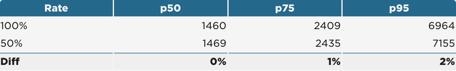
Aggregates: We will look at the percentage change between the 50th, 75th, and 95th percentiles. I considered anything under 5% acceptable.
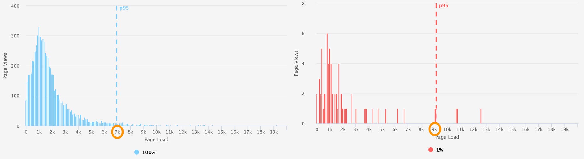
Histograms: You can learn a lot if you just look at your data. Histograms are great for showing the performance characteristics of an entire population. (Learn more about understanding and interpreting histograms.) For this experiment, we are comparing the overall shape and distribution of our sampled versus unsampled populations. In some cases, the aggregates may have been under 5%, but the the histogram was very sparse and didn't resemble the original distribution. For example, the differences between these two histograms is obvious despite their medians being within reason. When looking at the 95th percentile, you observe that the long tail is essentially 'missing' from the sampled data. While somewhat unscientific, I used the eyeball test along with the aggregates to decide if the rate was appropriate.
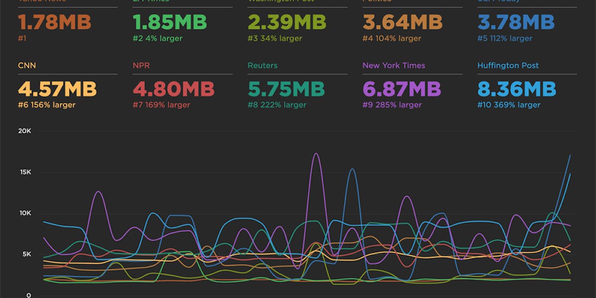
Time series: Intraday variability is important if you're using the RUM data operationally. A simple time series will be used to illustrate how sampling impacts the 'noise' factor.
Key findings
TL;DR
For the most part, I found that if the sampled population of users was greater than 3,000, the aggregate stats were pretty close to your upsampled population (1-2% difference in the median). However, you should read on to understand some of the trade-offs dependent on your use case for RUM. Or, if you'd rather, go ahead and jump to the results.
RUM for reporting
If you're simply looking to RUM as a reporting tool that can represent your daily performance, you're in luck. You can get away with a relatively small sample of your overall population depending on your size.
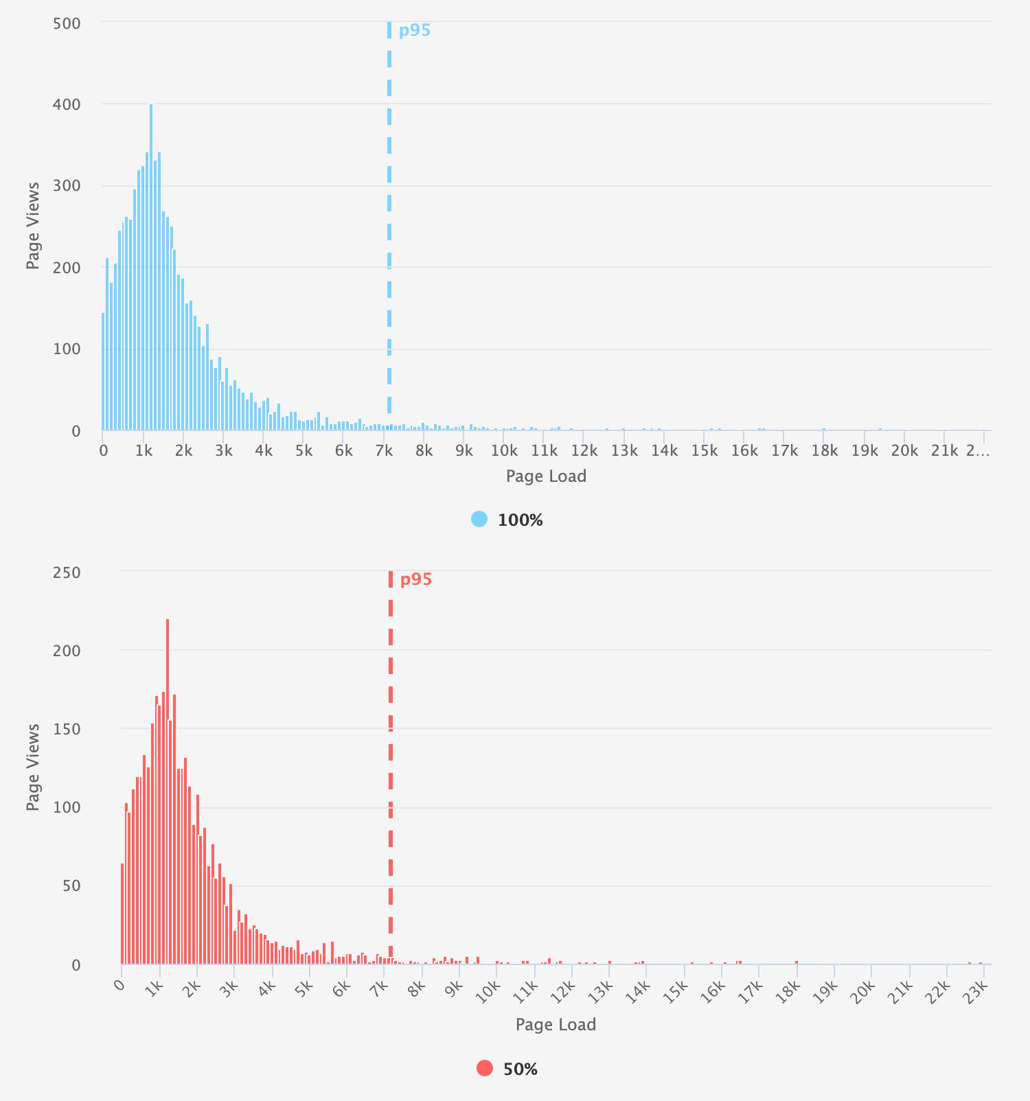
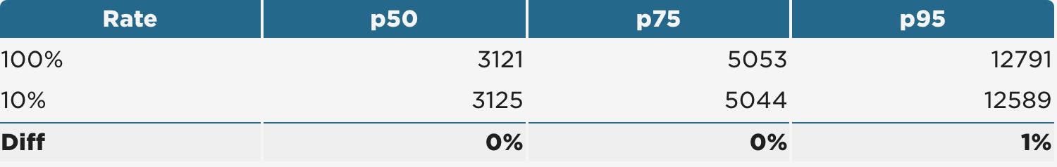
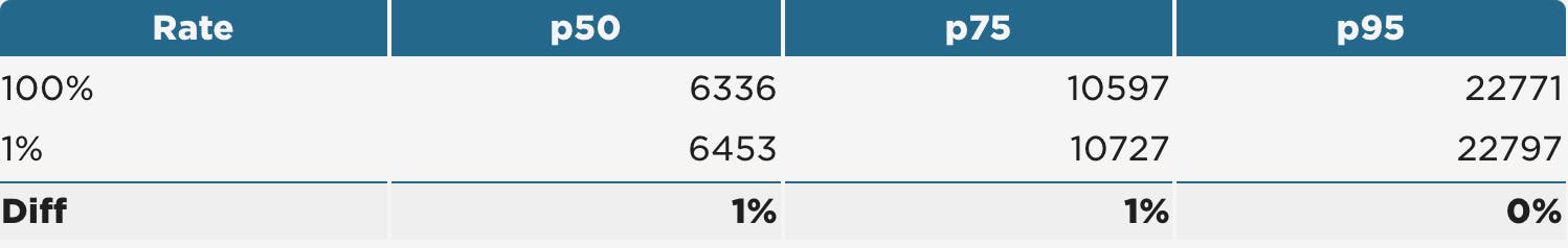
To determine the smallest sample rate for each group, we looked at a combination of the aggregate numbers and a comparison of the histograms. Note the consistency in the 95th percentile illustrated in these comparison charts.
Small (10K-100K daily page views sampled at 50%)
Medium (250K-500K daily page views sampled at 10%)
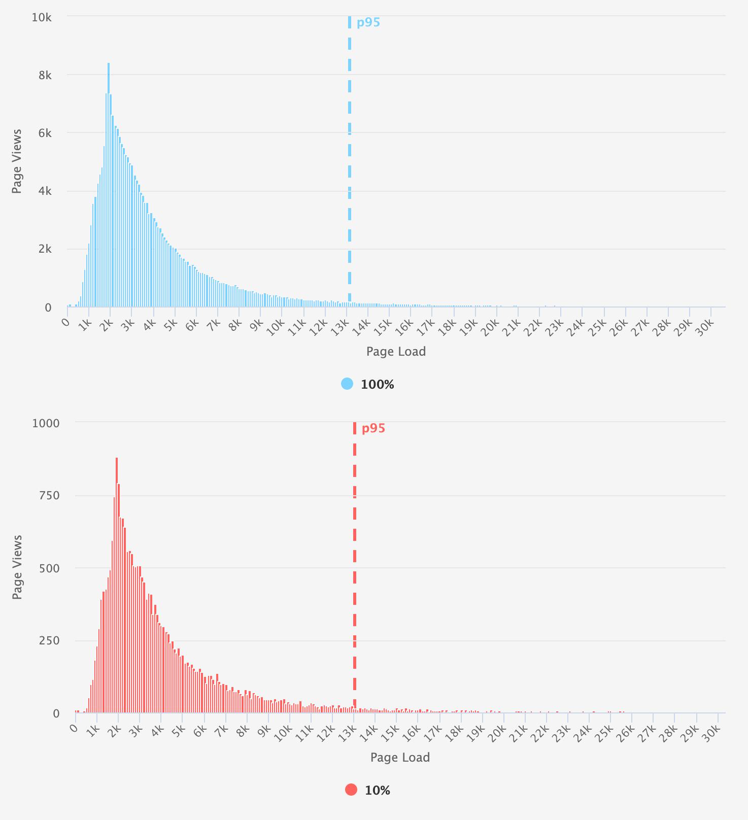
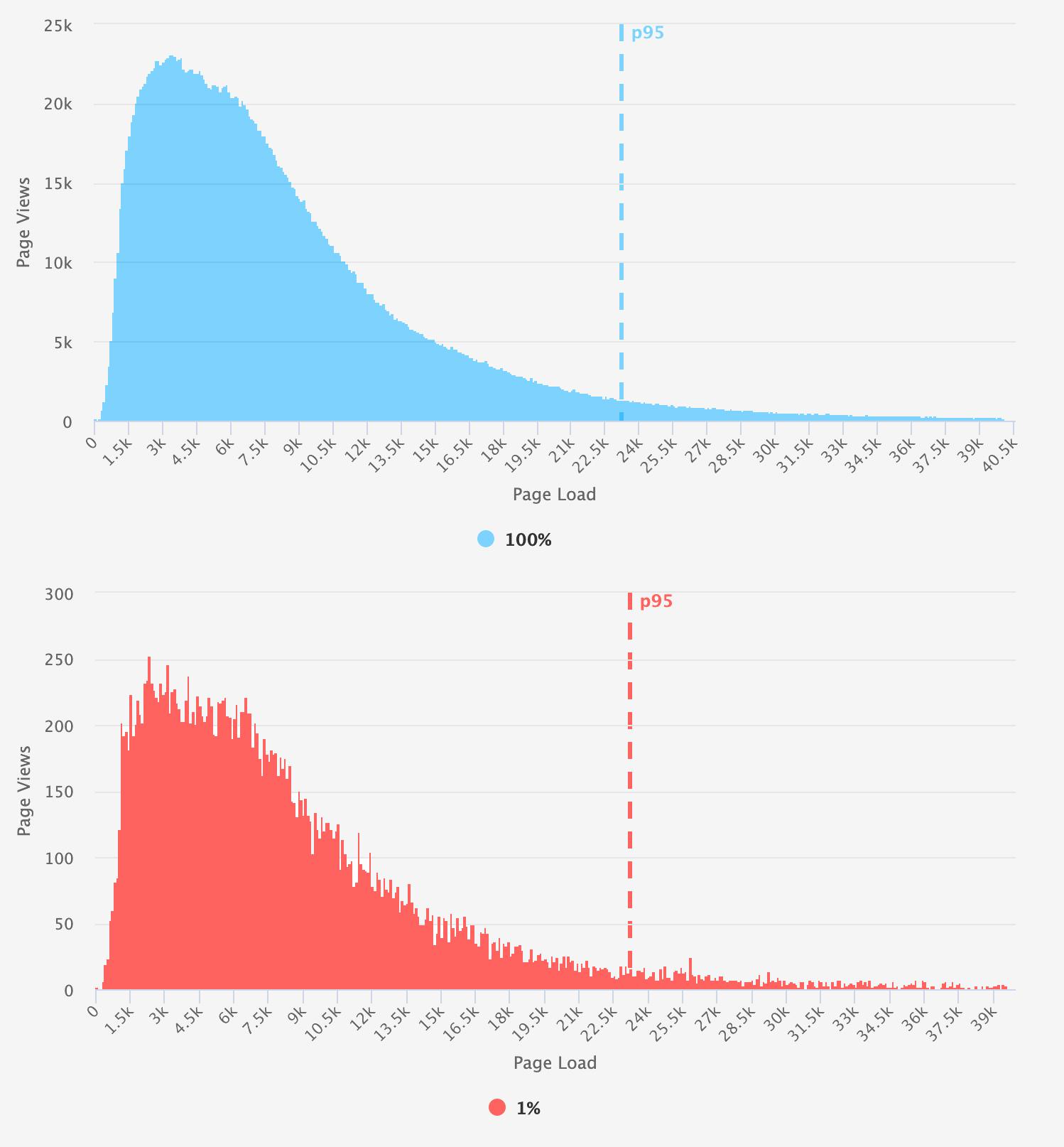
Large (>1M daily page views sampled at 1%)
Intraday performance monitoring
You might be one of those sites deploying code multiple times a day. Maybe you're susceptible to variability from things such as third parties, varying traffic patterns, or other unknowns. (Aren't we all?) If this is the case, you may have more operational need for RUM. Your sampling rate can have a bit of impact on whether or not your data appears noisy or unpredictable.
Looking at the recommended rates from the previous use case, the examples below show you how much you'll need to dial that up to get a reliable picture of hourly performance, and even more if you are looking at real-time monitoring (by minute).
Hourly monitoring:
Small – increased from 50% -> 75%

While increasing the rate helped remove some of the large deviations seen, the data is naturally much more variable for small-traffic sites.
Medium – increased from 10% -> 25%
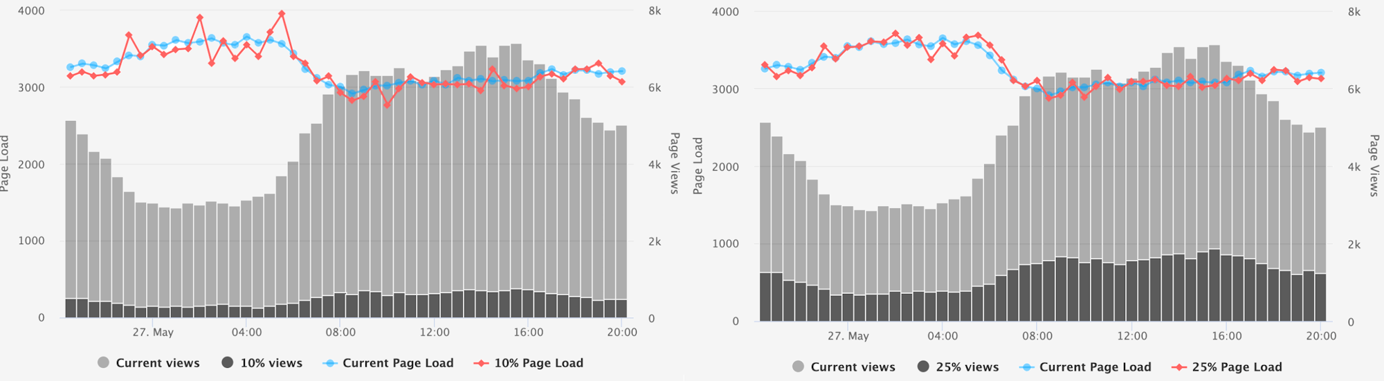
While the peak hours were somewhat consistent at 10%, increasing the rate to 25% removed the larger off-peak deviations.
Large – increased from 1% -> 10%
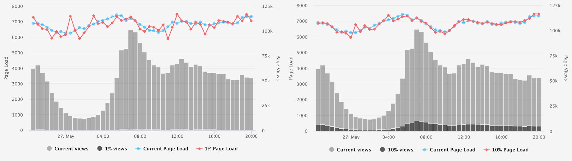
Increasing the rate by 10% greatly improved consistency for the large-traffic site.
Real-time monitoring:
Small – increased from 75% -> 95%

For some of the larger spikes in the data, increasing the sample to 95% was effective. However, given how variable the data is, it's hard to say if real-time monitoring of smaller sites like this is really very effective.
Medium – increased from 25% -> 75%

For the medium-traffic site, there was benefit when increasing the rate to 75%.
Large – increased from 10% -> 40%

For this particular large-traffic site, getting real-time data consistent with the whole population required a much larger increase in the sample rate than anticipated.
Considerations
Data segmentation
Here comes the kicker. One of the great things about RUM is the ability to slice and dice your data. The distribution of your user population is made up of all types of user experiences. This has a pretty big impact on your sample rate, as when you filter/segment/slice/dice your data, you're effectively reducing the size of your population.
When determining how sampling will be affected by the segments you care about, get an idea of the percentage of traffic that is represented by the segment and factor that percentage into your overall rate. Some of the common segments include country, page types, device types and browsers. After applying a lot of segmentation to the experiments above, a good rule of thumb is to increase your sample rate by 50% (or collect 100% of the data for small sites).
Metrics
As mentioned earlier, there are some metrics (okay, many metrics) that aren't supported across browsers. Just as you would increase your sample rate for the segments, you should consider increasing the sample rate for metrics such as FCP, LCP and Total Blocking Time, which don't have broad browser support. This is also true of some network-related metrics that don't occur on every page load (DNS, Connect, SSL, Redirect).
Increasing time windows
It's sometimes recommended that you need to capture 100% of your data if you are comparing RUM data for different experiments, or capturing conversion data in order to understand the business impact of performance. This is not always the case. As an alternative, you can look at a much larger time window with a LOT more sampled data. This is also true of sites with low traffic numbers. Simply expand your time window until you have a healthy distribution.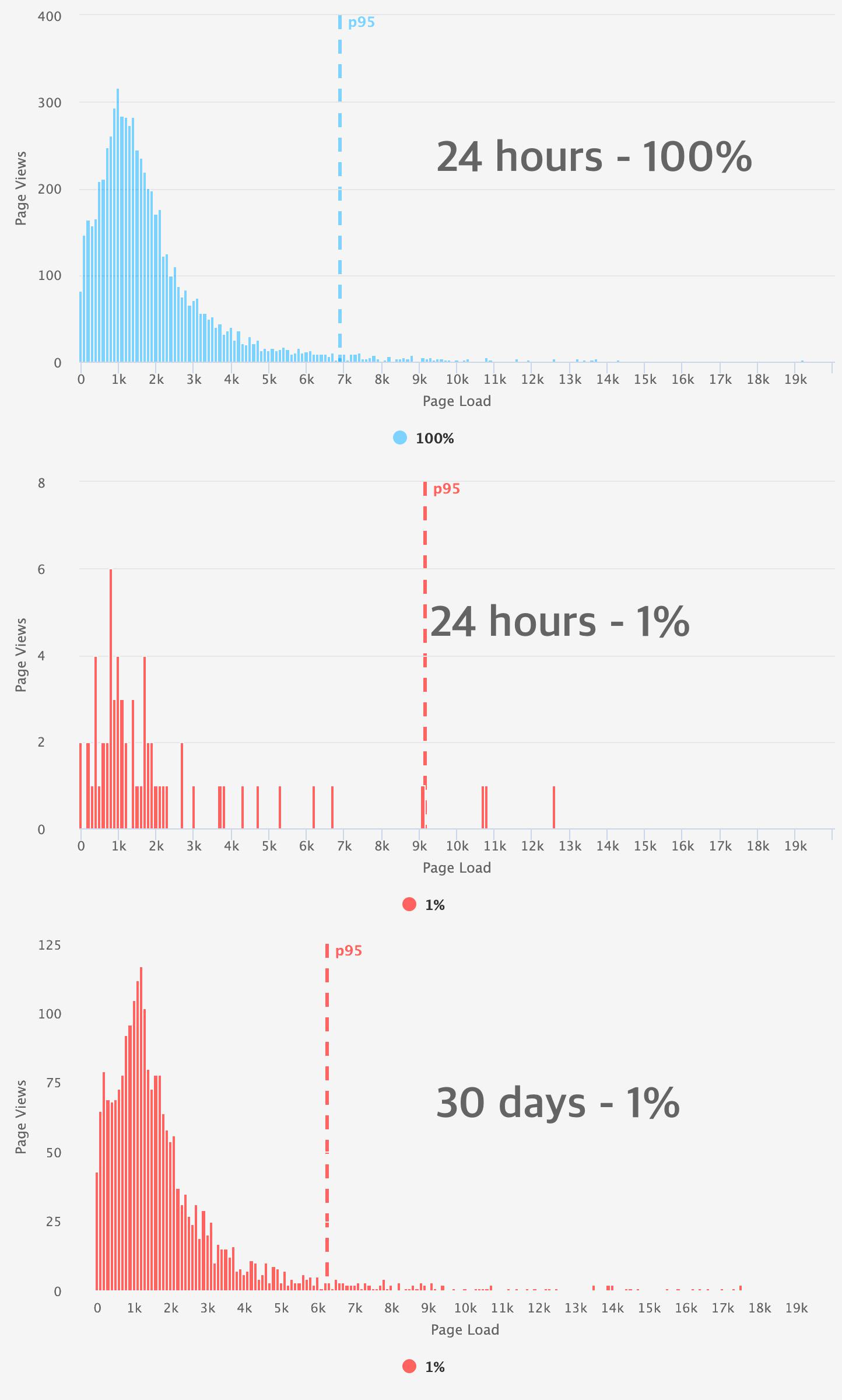
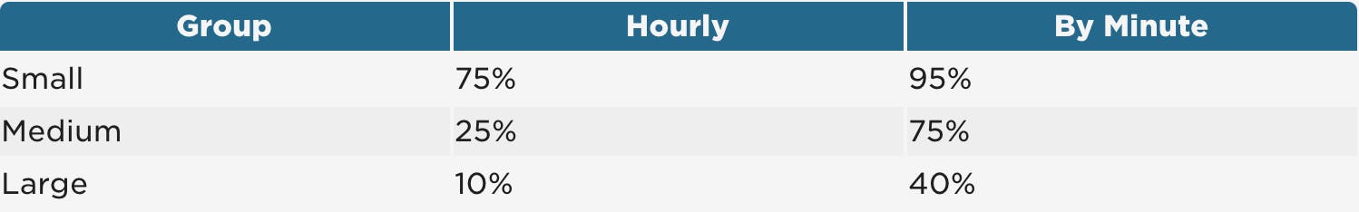
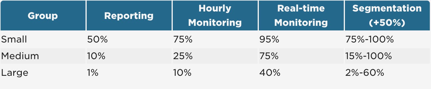
Recommendations
The intent of this post was to help provide some direction around sampling RUM data. The recommended levels are not intended to be precise, as there are too many factors that could influence things one way or the other. Use this table as a guide in addition to the knowledge you have about your users:
Learn more about RUM sampling
As you may have guessed, SpeedCurve supports data sampling in RUM. This article goes into detail about how our RUM sampling works and explains the different ways you can implement it. If you have any questions or feedback, we'd love to hear from you. Leave a comment below or send us a note at support@speedcurve.com.
Read Next

See how customers are using SpeedCurve to make their sites faster.
See industry-leading sites ranked on how fast their pages load from a user's perspective.