Beyond data and model parallelism for deep neural networks Jia et al., SysML’2019
I’m guessing the authors of this paper were spared some of the XML excesses of the late nineties and early noughties, since they have no qualms putting SOAP at the core of their work! To me that means the “simple” object access protocol, but not here:
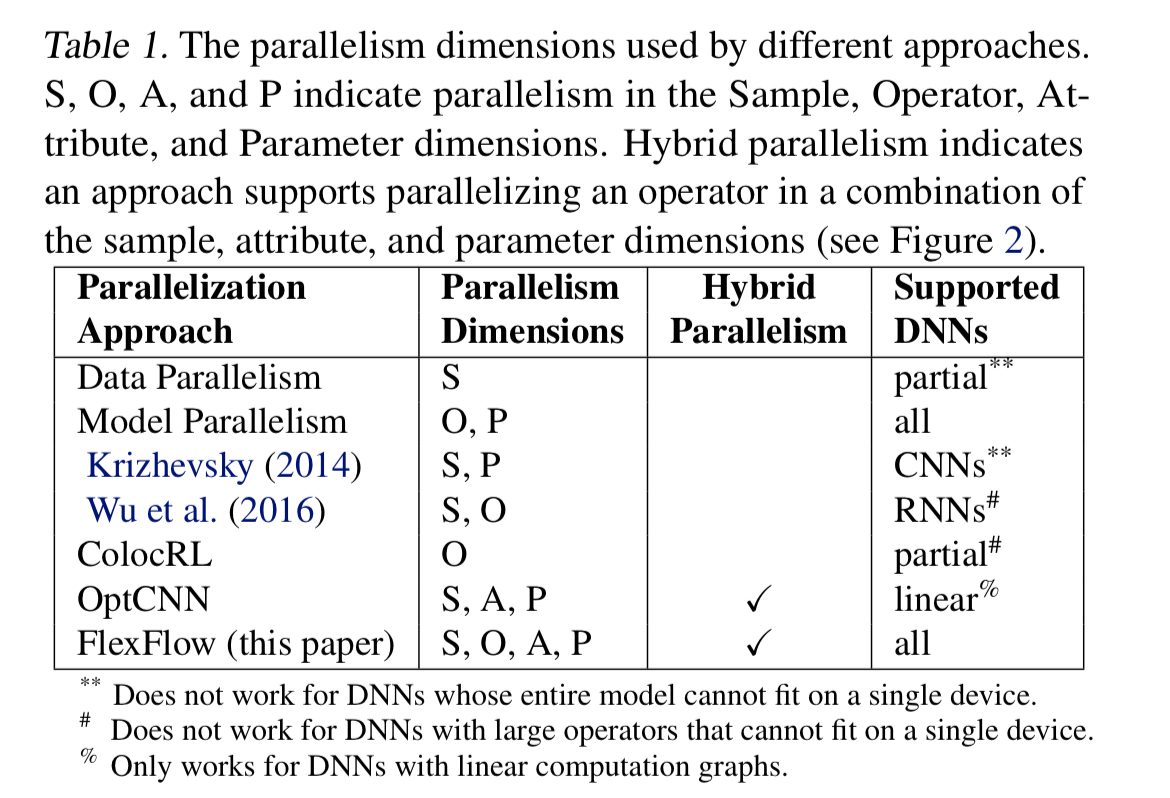
We introduce SOAP, a more comprehensive search space of parallelization strategies for DNNs that includes strategies to parallelize a DNN in the Sample, Operator, Attribute, and Parameter dimensions.
The goal here is to reduce the training times of DNNs by finding efficient parallel execution strategies, and even including its search time, FlexFlow is able to increase training throughput by up to 3.3x compared to state-of-the-art approaches.
There are two key ideas behind FlexFlow. The first is to expand the set of possible solutions (and hence also the search space!) in the hope of covering more interesting potential solutions. The second is an efficient execution simulator that makes searching that space possible by giving a quick evaluation of the potential performance of a given parallelisation strategy. Combine those with an off-the-shelf Metropolis-Hastings MCMC search strategy and Bob’s your uncle.
Expanding the search space
Traditional approaches to training exploit either data parallelism (dividing up the training samples), model parallelism (dividing up the model parameters), or expert-designed hybrids for particular situations. FlexFlow encompasses both of these in its sample (data parallelism), and parameter (model parallelism) dimensions, and also adds an operator dimension (more model parallelism) describing how operators within a DNN should be parallelised, and an attribute dimension with defines how different attributes within a sample should be partitioned (e.g. height and width of an image). Hence SOAP: Sample-Operator-Attribute-Parameter.
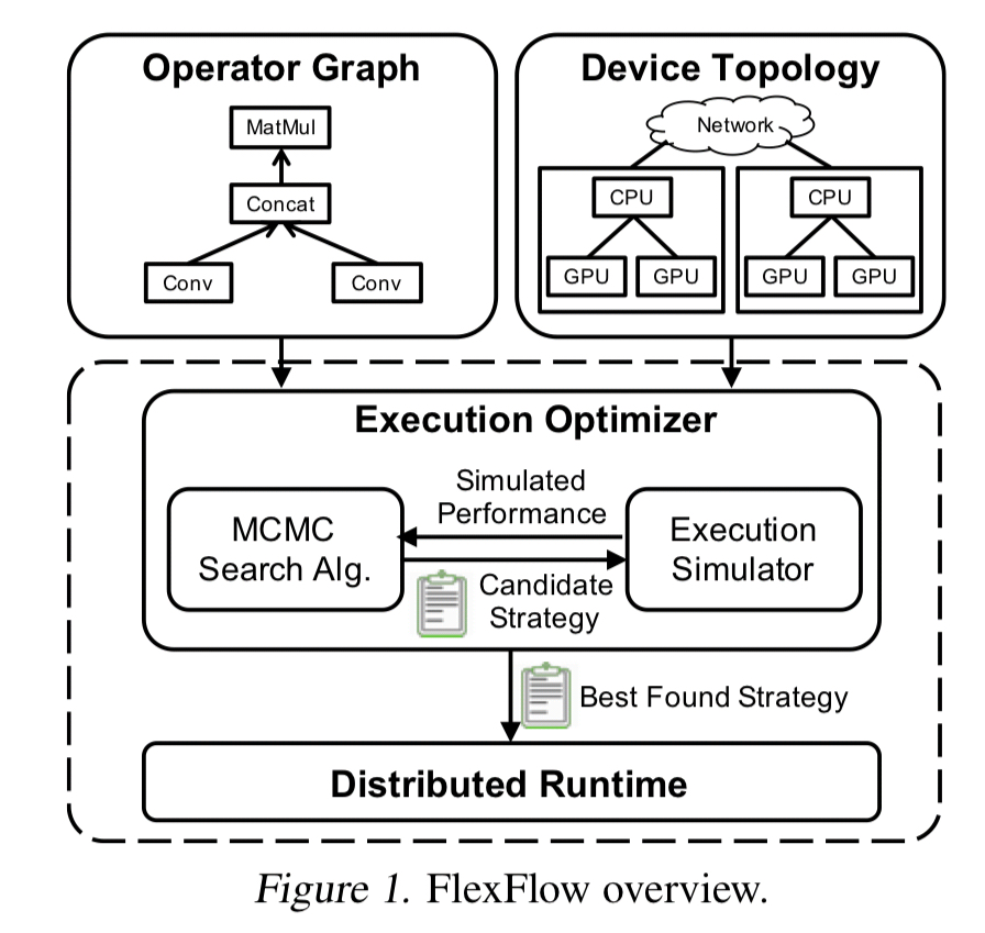
The input to FlexFlow is an operator graph describing all the operators and state in a DNN. Nodes are operators, and edges represent data flows of tensors. FlexFlow is also given a device topology graph describing all the available hardware devices and their interconnections.
To parallelize a DNN operator across device, we require each device to compute a disjoint subset of the operator’s output tensors. Therefore, we model the parallelization of an operator
by defining how the output tensor of
The parallelizable dimensions of an individual operator include the sample, attribute, and parameter dimensions. The operator dimension concerns parallelism across operators. A parallelization configuration defines how an operator is parallelized across multiple devices, including the degree of parallelism to be used in each dimension: an operator is partitioned into independent tasks, and tasks are assigned to devices. For example:
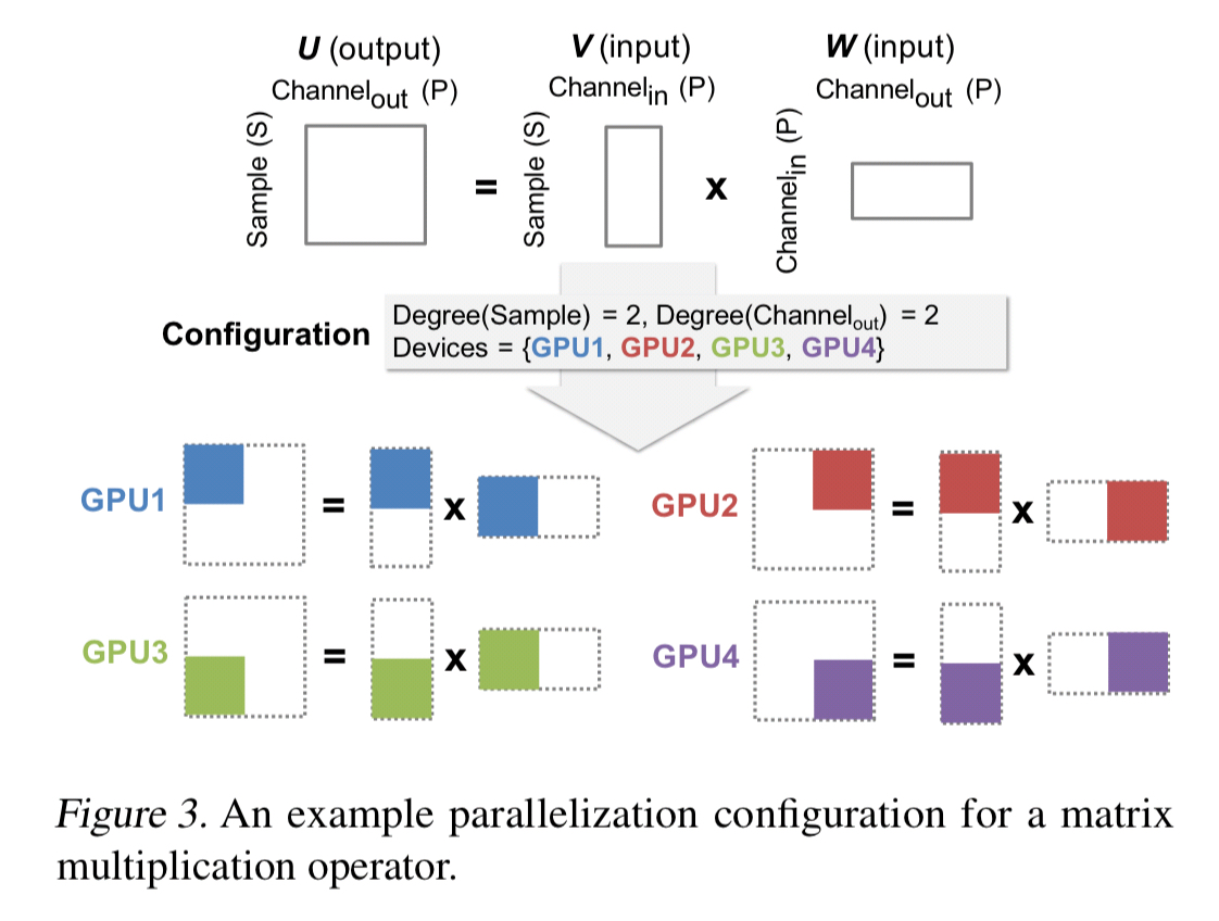
An overall parallelization strategy defines a parallelization configuration for each operator in the graph.
Execution simulation
The execution simulator takes an operator graph, a device topology, and a parallelization strategy as inputs, ad predicts the execution time.
…we borrow the idea from OptCNN to measure the execution time of each distinct operator once for each configuration and include these measurements in a task graph, which includes all tasks derived from operators and dependencies between tasks.
Hardware connections between devices are modelled as special communication devices which can execute communication tasks. This enables the whole execution time to be simulated using a single common abstraction.
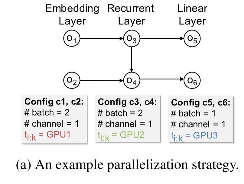
A typical parallelization strategy for a 3-layer RNN might look like this:
The corresponding task graph looks like this:

For a full simulation, a variant of Dijkstra’s shortest-path algorithm is used with tasks enqueued into a global priority queue when ready and dequeued in increasing order by their readyTime. The resulting execution timelines look like this (where r indicates the ready time, and s the start time).

While FlexFlow is exploring the search space, it changes the parallelization strategy of a single operator in each time step. Thus must of the task graph is unchanged from one simulation to the next.
Based on this observation, we introduce a delta simulation algorithm that starts from a previous task graph and only re-simulates tasks involved in the portion of the execution timeline that changes, an optimization that dramatically speeds up the simulator, especially for strategies for large distribution machines.
For example, suppose we reduce the parallelism of operator o3 down to 1. The task graph for the new resulting parallelization strategy requires updating only the simulation properties of the tasks in the grey shaded area below.

The optimiser
Finding the optimal parallelisation strategy is NP-hard, and the number of possible strategies is exponential in the number of operators in the graph. So exhaustive enumeration is out.
To find a low-cost strategy, FlexFlow uses a cost minimization search to heuristically explore the space and returns the best strategy discovered.
From a given initial strategy 

(Metropolis-Hastings)
 - cost(S*))})")
In other words, whenever the new strategy has equal or lower cost it is guaranteed to be accepted, but a strategy with higher cost may be accepted with likelihood controlled by the parameter 
Results
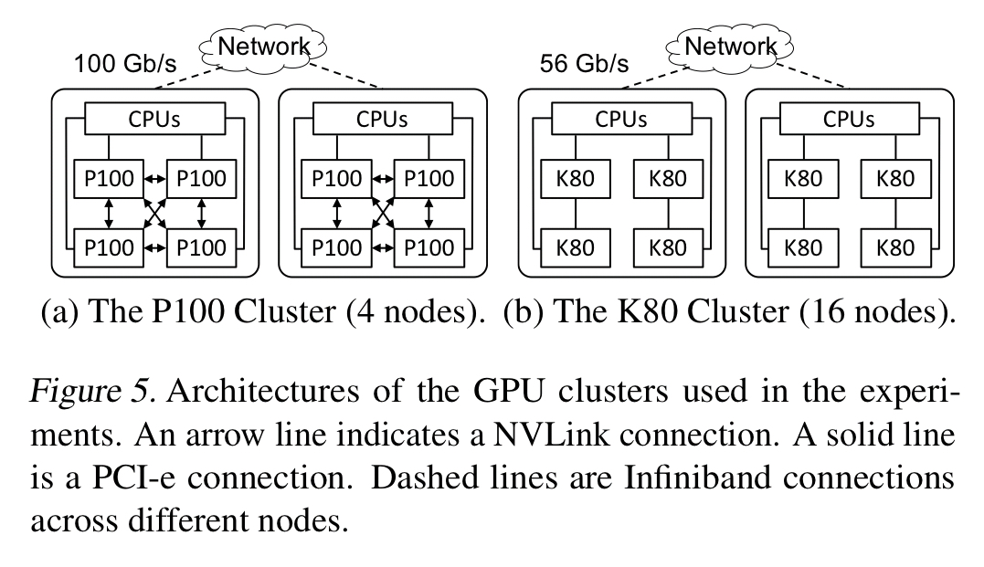
FlexFlow is evaluated over six real-world DNN benchmarks on two different GPU clusters.
The following charts show the training throughput for the best strategies found by FlexFlow, as compared to vanilla data parallelism or expert-defined strategies:
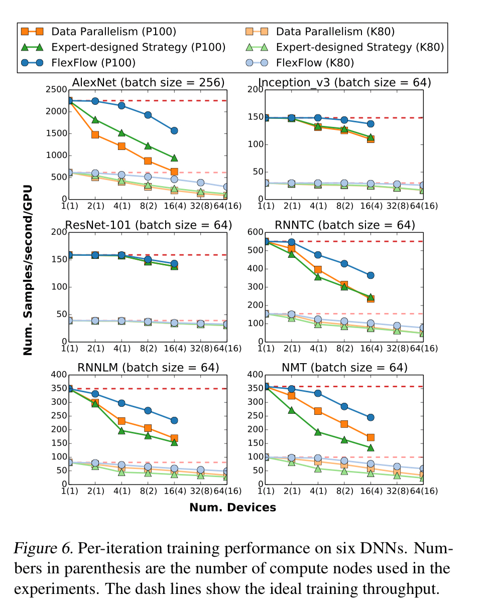
The strategies found by FlexFlow reduce per-iteration data transfers by 2-5.5x compared to other parallelisation strategies, and also reduce task computation time. Since it performs the same ultimate computation, the trained models have the same accuracy.
An evaluation of the execution simulator comparing estimated times to real execution times shows that the simulator is accurate to within 30%. Most importantly, the relative differences in simulated times mirror their real-world counterparts (i.e., if the simulator thinks a strategy will be better, it does turn out to be in practice).
Taking the NMT model as an example, the full simulation algorithm terminates in 16 minutes, and a search using delta simulation terminates in 6 minutes. If the time budget for searching is 8 minutes or less, the delta simulation algorithm finds the better solution.
So it all sounds very promising, but there is one big catch:
We found that existing deep learning systems (e.g. TensorFlow, PyTorch, Caffe2, and MXNet) only support parallelizing an operator in the sample dimension through data parallelism, and it is non-trivial to parallelize an operator in other dimensions or combinations of several SOAP dimensions in these systems.
The implementation in the paper uses Legion, cuDNN, and cuBLAS.